StatLit-Blog

Check out these news-story titles: How the average Brit has slept with 2.8 million people.   Ave Brit shagged 2.8 m people.  Someone is going to need a bigger bed.    Here’s one story:

Brits have had ‘indirect sex’ with 2.8 million people   (AFP) – Sep 23, 2009

LONDON – The average British man or woman has slept with 2.8 million people – albeit indirectly, according to figures released Wednesday to promote awareness of sexual health.  A British pharmacy chain has launched an online calculator which helps you work out how many partners you have had, in the sense of exposure to risk of sexually transmitted diseases (STIs).

The ‘Sex Degrees of Separation’ ready reckoner tots up the numbers based on your number of partners, then their previous partners, and their former lovers, and so on for six ‘generations’ of partners.  The average British man claims to have actually slept with nine people, while women put the figure at 6.3, giving an average of 7.65.

‘When we sleep with someone, we are, in effect, not only sleeping with them, but also their previous partners and their partners’ previous partners, and so on,’ said Ms Clare Kerr, head of sexual health at Lloydspharmacy.  ‘It’s important that people understand how exposed they are to STIs and take appropriate precautions including using condoms and getting themselves checked out where appropriate.’

Now my side of the story.  Lloyds has created a “statistically transmitted disease.”  This disease is transmitted via sexual contact but these sexual contacts are based on a model — a statistical model.  Lloyds goes out six generations beyond your immediate partners.  This choice is totally arbitrary.  The more generations out, the bigger the number.  Lloyd’s model gets a big number by being unrealistic.

Lloyd’s model ignores five big items: the prevalence, communicability and remoteness of the disease, the order in which the sexual contacts occur, and the inappropriateness of the average. 

After taking into account the five things Lloyds ignored, I estimate the Lloyd’s number is ten thousand times as big as any sexually-relevant number.  Instead of 2.8 million, I estimate 280 sexually-relevant partners.

(1)  PREVALENCE:  If only 20% of adults have STDs, then the number of sexually-relevant partners is less by a factor of five. 

(2)  COMMUNICABILITY and (3) REMOTENESS:  The Lloyds model assumes that everyone who has sex with someone having a STD will catch that disease.  This is unrealistic.  Suppose there is a 10% chance of catching an STD from a partner that has it.  The chance of acquiring an STD from someone six generations away is miniscule.  Averaging over the varying degrees of separation might give a total number of sexually-relevant partners that is less by a factor of at least a hundred. 

(4)  ORDER:  To measure vulnerability to sexually-transmitted diseases, the issue is not how many sexual partners your partners had, but which events occurred first so that diseases could be transmitted to you.  The Lloyd’s reckoner assumes that order is irrelevant.  I’m guessing that taking into account all possible orderings to get the number of indirect sexual partners that could transmit disease could give a total number of sexually-relevant partners that is less by a factor of two or three.

(5)  AVERAGE:  The Lloyd’s reckoner uses averages.  This number-of-partners distribution is highly skewed.  There are more “rabbits” than virgins and some rabbits are very “promiscuous.”  Those promiscuous rabbits will pull the mean quite a ways above the median.  Assuming you and your sexual partners are not highly promiscuous, this choice is likely to persist through your chain of sexual partners.  In such a case, the median is more appropriate.  If the median is 70% of the mean, then the seven-generation estimate is 0.7 to the seventh power of the original: 0.08 – a ten-fold reduction.  If the median is 50% of the mean, then the seven-generation estimate is 0.5 to the seventh power of the original: 0.008 – a hundred-fold reduction.

Summary:  Making all these adjustments gives a total number of relevant partners that is less by a factor of 10,000: going from 2.8 million to 280.  If we’re going to have a statistically-transmitted disease, it should be modeled realistically.   

More technical details here and here.  OK numbers people.  What do you make of Lloyd’s reckoner and these adjustments?

10/22/09: The Associated Press (AP) released a story, Belief in Global Warming is Cooling, that said:

• 57% of Americans said [yes] there is solid evidence that the earth is warming [a 14 point drop from 2008]
• 36% [of Americans] said temperatures are rising because of human activity [an 11 point drop from 2008]

 The AP also released this graph (AP ID: 09102201574) that described the 36% differently:

• 36% of those who answered yes, said temperatures are rising because of human activity. 

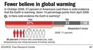
Now, 36% of 57% is around 20%.   So according to this AP graph, only 20% of Americans said temperatures are rising because of human activity.  This 20% would be big news if it were true.    Both AP interpretations of the 36% came from this table. 

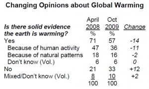
Source: Fewer Americans See Solid Evidence of Global Warming by The Pew Research Center for the People & the Press.   Notice that this table is a multi-level percentage table: the percentages add to more than the totals and some of the rows are indented.  Percentage tables are not always easy to read – even by professionals.

 On 10/23, the AP released a second graph (AP ID: 0910222617) that deleted the 36% description used in their first graph.  

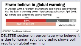
Did the AP make the right decision?   What do you think and why?

Read the rest of this entry »

Comparisons of SAT scores within a given year are pretty-much meaningless. Comparisons of percentiles are much more meaningful.

Consider the 2009 SAT Math scores presented in an Economix blog:
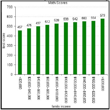The higher the family income, the higher the average score math score.  But how big is this difference.  Yes, 122 points between the extremes.  But so what? What does 122 points mean?

If one knows the possible range of scores (200 to 800), one can make some comparison.  But this isn’t very helpful.

Another technique is to make a percentage comparison. Here the top score (579) is 27% more the bottom score (457).    But this comparison is meaningless.  SAT scores are arbitrary.  They are selected to range from 200 to 800 – a factor of four or a difference of 300%.  If we added 1,000 to each score, they would range from 1200 to 1800 – a factor of 1.5 or a difference of 50%.  By focusing on arbitrary scores, this graph promotes statistical illiteracy. 

We need a better way to put scores in context.   Consider this: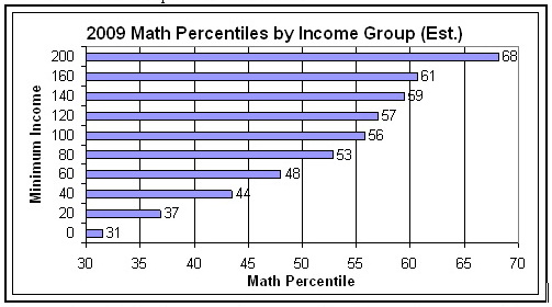These values are percentiles.  Percentiles are not arbitrary;  they provide their own context.  In this case, scores range from the 31-st percentile to the 68-th percentile.  The high-low income SAT Math gap is 37 percentiles. 

Anyone reading this graph can immediately see how much the SAT Math scores are influenced by family income — or by income related factors.

Why didn’t the blogger present the scores in this fashion.  The College Board provides data by family incomes as SAT scores – not by percentiles.  Also, the College Board doesn’t provide a convenient way to convert SAT scores to percentiles. 

Recommendation: The College Board should give their results as SAT scores AND as percentiles – or give a way to convert SAT scores into percentiles.

Sources:
Blog:  http://economix.blogs.nytimes.com/2009/08/27/sat-scores-and-family-income/
Data:  http://professionals.collegeboard.com/profdownload/SAT-Percentile-Ranks-2009.pdf

On Sept 30, the AP claimed that 69% of candy-eating kids become criminals.  Like most AP stories, this one appeared in dozens of papers.   The only problem was this claim was false.  Here is the Associated Press (AP) story:

AP: Sept 30 2009.  Study says too much candy could lead to prison

LONDON, England — Willy Wonka would be horrified. Children who eat too much candy may be more likely to be arrested for violent behavior as adults, new research suggests.

British experts studied more than 17,000 children born in 1970 for about four decades. Of the children who ate candies or chocolates daily at age 10, 69 percent were later arrested for a violent offense by the age of 34. Of those who didn’t have any violent clashes, 42 percent ate sweets daily.

The AP single-handedly upped the violent crime rate for candy-eating kids from 0.8% in reality to 69% in their story.  The  AP has unleashed the tsunami of all crime waves.

This 69% bogus statistic was carried by MSNBC, CBS News, Fox News, Forbes, Google and Yahoo.

The AP statement is false and wildly so.  Look at the numbers:
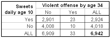
*  Of the 17,000 children in the project, 6,942 fit this study.
*  Of these 6,942 kids, 2,924 (42%) had candy daily at age 10.
*  Of the 2,924 kids, 23 (0.8%) had violence convictions by age 34

Note the difference:  0.8% of candy-eaters arrested in the actual data vs. 69% of candy-eaters arrested in the AP story.   Candy is not good for the teeth, but it hardly seems adequate to cause 69% of sweet-eating kids to become violent offenders by age 34.  Once again statistical illiteracy strikes journalists.

So where did the AP get the 69%?  From the original article.   Here is the relevant piece:

Results: Overall, 69% of respondents who were violent by the age of 34 years reported that they ate confectionary nearly every day during childhood, compared with 42% who were non-violent.

Confectionary consumption in childhood and adult violence by Moore et al, The British Journal of Psychiatry, 2009 195: 366-367

The AP took the 69% ratio and switched part and whole.  Compare the whole in the journal article with that in the AP story:
* Journal: respondents who were violent by the age of 34 years
* AP:  children who ate candies or chocolates daily at age 10
The AP is guilty of confusing the inverse: P(A|B) = P(B|A).

If you need more detail, the journal article included this:
“The binary outcome variable, violence, is a rare event (0.47%)”  “Observations n = 6,942.”  Combining their results gives this table:

Q1.  Should the AP retract their bad statistic?
Q2. Would most readers understand the difference?